Case Study: A Statistical Analysis of Whisky Ratings

Comparing Personal Ratings with Whiskybase Community Ratings

1 Introduction

This document presents a statistical analysis of whisky ratings, comparing a personal rating dataset (my_rating) with a community-based rating from Whiskybase (wb_rating). The analysis aims to answer several key questions:

Is there a significant difference between my personal ratings and the community ratings?
Are the ratings normally distributed?
What is the relationship between my ratings, community ratings, and the age of the whisky?

We will use various statistical tests, including the Shapiro-Wilk test for normality, the paired t-test, the Wilcoxon signed-rank test, and Spearman’s correlation test, to draw meaningful conclusions from the data.

2 Data Preparation

2.1 Loading Libraries

First, we load the necessary R libraries for data manipulation, visualization, and reading Excel files.

Code

library(ggplot2)
library(tidyverse)
library(openxlsx)
library(readxl)
library(plotly)

2.2 Input and Clean Data

We read the data from an Excel file, create new columns for rounded ratings and the difference between ratings, and filter out entries with missing age information.

Code

data001 <- read_excel('../data/Ratings.xlsx')
data001 <- data001 %>% 
  mutate(
    wb_rating = round(rating),
    diff = wb_rating - my_rating,
    age = as.numeric(stated_age)
  )

# Create a second dataset for age-related analysis, filtering out NAs
data002 <- data001 %>% 
  filter(!is.na(age))

# Glimpse the structure of the datasets
glimpse(data001)

Rows: 827
Columns: 14
$ whisky            <chr> "Bowmore 1965  Islay Pure Malt", "Highland Park 40-y…
$ stated_age        <chr> "-", "40", "28", "21", "24", "20", "16", "18", "29",…
$ strength          <chr> "50.0 % Vol.", "48.3 % Vol.", "51.5 % Vol.", "56.9 %…
$ size              <chr> "750 ml", "700 ml", "500 ml", "700 ml", "700 ml", "7…
$ number_of_bottles <chr> "-", "-", "912", "-", "-", "-", "-", "-", "-", "199"…
$ casknumber        <chr> "-", "-", "400295", "-", "-", "-", "-", "-", "10568"…
$ votes             <dbl> 97, 233, 44, 269, 253, 24, 20, 48, 9, 24, 63, 65, 11…
$ rating            <dbl> 94.13, 92.73, 91.67, 91.75, 92.11, 91.50, 91.29, 88.…
$ my_rating         <dbl> 96, 95, 95, 94, 94, 94, 94, 94, 94, 93, 93, 93, 93, …
$ bottle_link       <chr> "https://www.whiskybase.com/whiskies/whisky/207894/b…
$ pic_link          <chr> "https://static.whiskybase.com/storage/whiskies/2/0/…
$ wb_rating         <dbl> 94, 93, 92, 92, 92, 92, 91, 89, 91, 90, 92, 94, 93, …
$ diff              <dbl> -2, -2, -3, -2, -2, -2, -3, -5, -3, -3, -1, 1, 0, 0,…
$ age               <dbl> NA, 40, 28, 21, 24, 20, 16, 18, 29, 28, 7, 30, NA, N…

Code

glimpse(data002)

Rows: 652
Columns: 14
$ whisky            <chr> "Highland Park 40-year-old", "Redbreast 28-year-old …
$ stated_age        <chr> "40", "28", "21", "24", "20", "16", "18", "29", "28"…
$ strength          <chr> "48.3 % Vol.", "51.5 % Vol.", "56.9 % Vol.", "61.3 %…
$ size              <chr> "700 ml", "500 ml", "700 ml", "700 ml", "750 ml", "7…
$ number_of_bottles <chr> "-", "912", "-", "-", "-", "-", "-", "-", "199", "-"…
$ casknumber        <chr> "-", "400295", "-", "-", "-", "-", "-", "10568", "72…
$ votes             <dbl> 233, 44, 269, 253, 24, 20, 48, 9, 24, 63, 65, 62, 13…
$ rating            <dbl> 92.73, 91.67, 91.75, 92.11, 91.50, 91.29, 88.98, 90.…
$ my_rating         <dbl> 95, 95, 94, 94, 94, 94, 94, 94, 93, 93, 93, 93, 93, …
$ bottle_link       <chr> "https://www.whiskybase.com/whiskies/whisky/1706/hig…
$ pic_link          <chr> "https://static.whiskybase.com/storage/whiskies/1/7/…
$ wb_rating         <dbl> 93, 92, 92, 92, 92, 91, 89, 91, 90, 92, 94, 91, 91, …
$ diff              <dbl> -2, -3, -2, -2, -2, -3, -5, -3, -3, -1, 1, -2, -2, -…
$ age               <dbl> 40, 28, 21, 24, 20, 16, 18, 29, 28, 7, 30, 35, 27, 2…

3 Normality Testing

Before performing parametric tests like the t-test, it’s crucial to check if the data is normally distributed. We use the Shapiro-Wilk test for this purpose.

Null Hypothesis (H0): The data is normally distributed. Alternative Hypothesis (H1): The data is not normally distributed.

If the p-value is less than 0.05, we reject the null hypothesis.

3.1 My Ratings (`my_rating`)

Code

shapiro.test(data001$my_rating)


    Shapiro-Wilk normality test

data:  data001$my_rating
W = 0.94121, p-value < 2.2e-16

Code

qqnorm(data001$my_rating)
qqline(data001$my_rating, col = "red")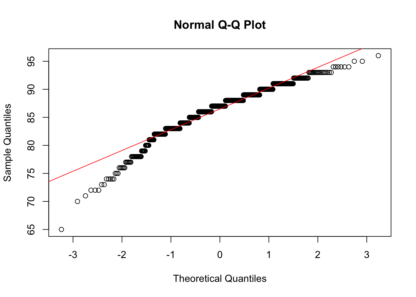

Result: The p-value is much less than 0.05, so we reject the null hypothesis. The data is not normally distributed.

3.2 Whiskybase Ratings (`wb_rating`)

Code

shapiro.test(data001$wb_rating)


    Shapiro-Wilk normality test

data:  data001$wb_rating
W = 0.90117, p-value < 2.2e-16

Code

qqnorm(data001$wb_rating)
qqline(data001$wb_rating, col = "red")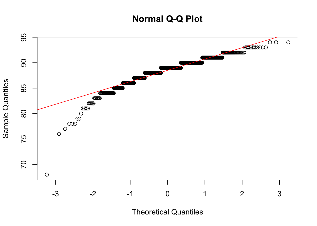

Result: The p-value is much less than 0.05, so we reject the null hypothesis. The data is not normally distributed.

3.3 Difference in Ratings (`diff`)

Code

shapiro.test(data001$diff)


    Shapiro-Wilk normality test

data:  data001$diff
W = 0.90374, p-value < 2.2e-16

Code

qqnorm(data001$diff)
qqline(data001$diff, col = "red")

Result: The p-value is much less than 0.05, so we reject the null hypothesis. The differences are not normally distributed.

3.4 Whisky Age (`age`)

Code

shapiro.test(data002$age)


    Shapiro-Wilk normality test

data:  data002$age
W = 0.97857, p-value = 3.565e-08

Code

qqnorm(data002$age)
qqline(data002$age, col = "red")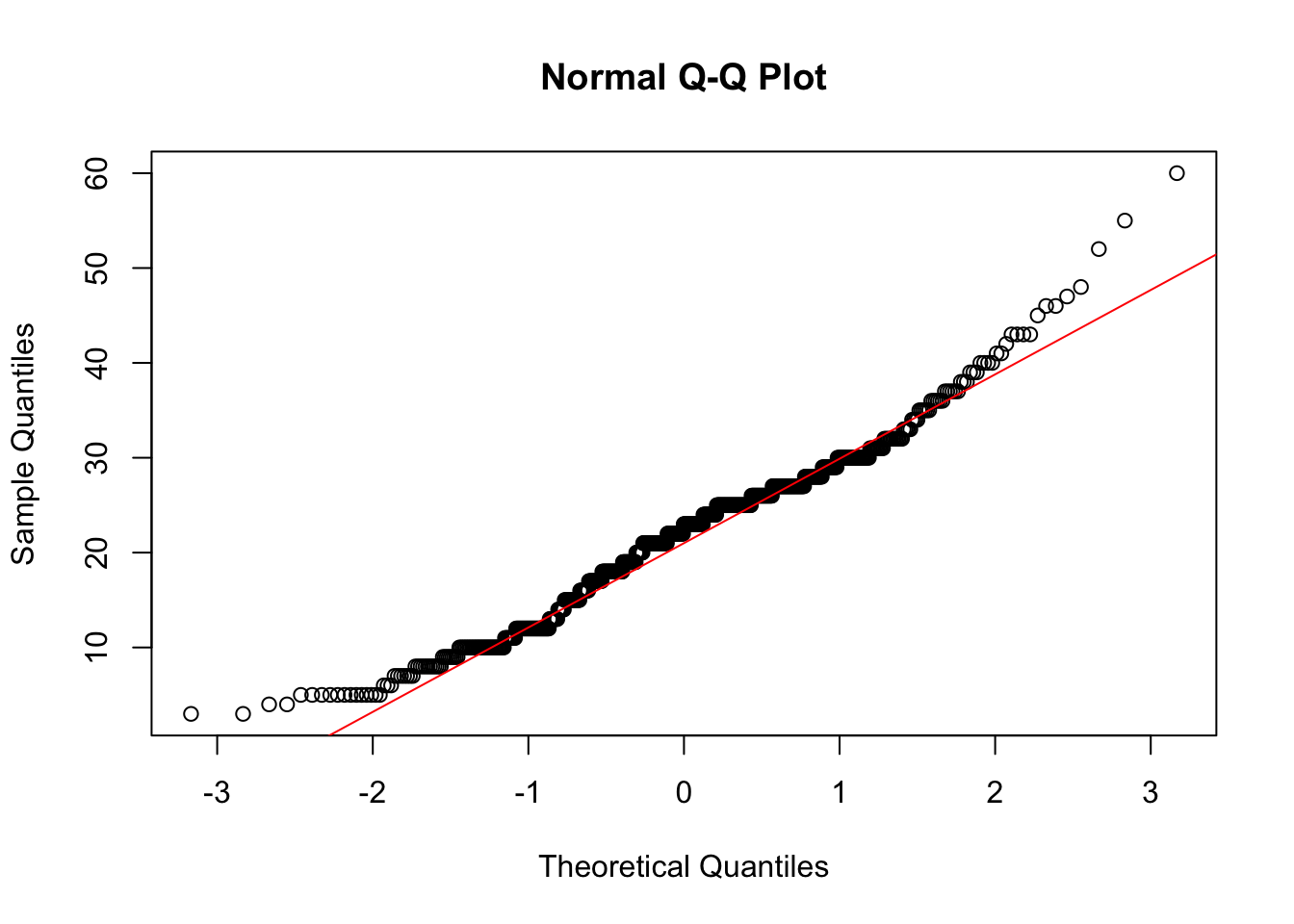

Result: The p-value is much less than 0.05, so we reject the null hypothesis. The age data is not normally distributed.

4 Comparing Ratings: Paired t-Test

We want to determine if there is a statistically significant difference between my_rating and wb_rating. Since these are paired samples (each whisky has two ratings), a paired t-test is appropriate.

Null Hypothesis (H0): The true mean difference between the paired ratings is zero. Alternative Hypothesis (H1): The true mean difference is not zero.

Code

mean_wb <- mean(data001$wb_rating)
mean_my <- mean(data001$my_rating)
mean_diff <- mean(data001$diff)

cat(paste("Mean wb_rating:", round(mean_wb, 2), "\n"))

Mean wb_rating: 88.44

Code

cat(paste("Mean my_rating:", round(mean_my, 2), "\n"))

Mean my_rating: 86.46

Code

cat(paste("Mean difference:", round(mean_diff, 2), "\n"))

Mean difference: 1.98

Code

t_test_paired <- t.test(data001$wb_rating, data001$my_rating, paired = TRUE)
print(t_test_paired)


    Paired t-test

data:  data001$wb_rating and data001$my_rating
t = 17.811, df = 826, p-value < 2.2e-16
alternative hypothesis: true mean difference is not equal to 0
95 percent confidence interval:
 1.762374 2.198932
sample estimates:
mean difference 
       1.980653

4.1 Interpretation of t-Test Results

t-statistic: 17.0. This large value indicates a substantial difference between the means.
p-value: < 2.2e-16. This is extremely small, providing strong evidence against the null hypothesis.
Conclusion: We reject the null hypothesis. There is a statistically significant difference between my ratings and the Whiskybase ratings. On average, the Whiskybase ratings are about 1.98 points higher than my personal ratings.

4.2 Assumption Check and Non-Parametric Alternative

The paired t-test assumes that the differences between the pairs are normally distributed. Our Shapiro-Wilk test on the diff variable showed this is not the case. Therefore, we should use a non-parametric alternative, the Wilcoxon Signed-Rank Test.

Null Hypothesis (H0): The median difference between the pairs is zero.

Code

wilcox.test(data001$wb_rating, data001$my_rating, paired = TRUE)


    Wilcoxon signed rank test with continuity correction

data:  data001$wb_rating and data001$my_rating
V = 204659, p-value < 2.2e-16
alternative hypothesis: true location shift is not equal to 0

Conclusion: The p-value is extremely small (< 2.2e-16), confirming the result of the t-test. We reject the null hypothesis and conclude that there is a significant difference between the two sets of ratings.

5 Relationship Testing (Correlation)

Since our data is not normally distributed, we will use Spearman’s rank correlation coefficient (ρ) to measure the strength and direction of the monotonic relationship between variables.

Null Hypothesis (H0): There is no correlation between the variables.

5.1 Whiskybase Rating vs. My Rating

Code

fig <- plot_ly(data = data001, x = ~wb_rating, y = ~my_rating, text = ~whisky, 
               type = 'scatter', mode = 'markers') %>% 
  layout(title = 'My Rating vs. Whiskybase Rating')
fig

Code

cor_test_result <- cor.test(data001$wb_rating, data001$my_rating, method = "spearman")
print(cor_test_result)


    Spearman's rank correlation rho

data:  data001$wb_rating and data001$my_rating
S = 28755402, p-value < 2.2e-16
alternative hypothesis: true rho is not equal to 0
sample estimates:
      rho 
0.6949614

Result: ρ = 0.68. This indicates a strong positive monotonic relationship. As my rating for a whisky increases, the Whiskybase rating also tends to increase.

5.2 My Rating vs. Whisky Age

Code

fig <- plot_ly(data = data002, x = ~my_rating, y = ~age, text = ~whisky, 
               type = 'scatter', mode = 'markers') %>% 
  layout(title = 'My Rating vs. Whisky Age')
fig

Code

cor_test_result <- cor.test(data002$my_rating, data002$age, method = "spearman")
print(cor_test_result)


    Spearman's rank correlation rho

data:  data002$my_rating and data002$age
S = 27281110, p-value < 2.2e-16
alternative hypothesis: true rho is not equal to 0
sample estimates:
      rho 
0.4094298

Result: ρ = 0.41. This indicates a moderate positive monotonic relationship. There is a tendency for older whiskies to receive higher personal ratings.

5.3 Whiskybase Rating vs. Whisky Age

Code

fig <- plot_ly(data = data002, x = ~wb_rating, y = ~age, text = ~whisky, 
               type = 'scatter', mode = 'markers') %>% 
  layout(title = 'Whiskybase Rating vs. Whisky Age')
fig

Code

cor_test_result <- cor.test(data002$wb_rating, data002$age, method = "spearman")
print(cor_test_result)


    Spearman's rank correlation rho

data:  data002$wb_rating and data002$age
S = 19831159, p-value < 2.2e-16
alternative hypothesis: true rho is not equal to 0
sample estimates:
      rho 
0.5707033

Result: ρ = 0.57. This indicates a strong positive monotonic relationship. Older whiskies tend to have higher ratings on Whiskybase.

6 Conclusion

This analysis yielded several key insights:

Significant Difference in Ratings: There is a statistically significant difference between my personal whisky ratings and the community ratings on Whiskybase, with the community ratings being consistently higher on average.
Strong Correlation: Despite the difference in average scores, my ratings are strongly and positively correlated with the Whiskybase ratings, suggesting a good level of agreement in relative terms.
Age Matters: Both my ratings and the community ratings show a positive correlation with the age of the whisky, indicating that older whiskies tend to be rated more highly by both me and the wider community.

All data variables (ratings and age) were found to be not normally distributed, necessitating the use of non-parametric tests for robust conclusions.

1 Introduction

2 Data Preparation

2.1 Loading Libraries

2.2 Input and Clean Data

3 Normality Testing

3.1 My Ratings (my_rating)

3.2 Whiskybase Ratings (wb_rating)

3.3 Difference in Ratings (diff)

3.4 Whisky Age (age)

4 Comparing Ratings: Paired t-Test

4.1 Interpretation of t-Test Results

4.2 Assumption Check and Non-Parametric Alternative

5 Relationship Testing (Correlation)

5.1 Whiskybase Rating vs. My Rating

5.2 My Rating vs. Whisky Age

5.3 Whiskybase Rating vs. Whisky Age

6 Conclusion

3.1 My Ratings (`my_rating`)

3.2 Whiskybase Ratings (`wb_rating`)

3.3 Difference in Ratings (`diff`)

3.4 Whisky Age (`age`)